LearnSeurat_PBMC3k
本系列假定读者对于单细胞测序的数据分析和Seurat的官方教程有所了解。
本篇研究最基础的PBMC3k。其实这里只有2700个外周血的细胞。注意到,由于取样是外周血,没有干细胞的存在,所以可以认为样品处于稳态。这个教程就是讲稳态下的单细胞测序分析是如何进行的。Seurat的官方教程的缺点之一就是没有涉及动态过程的单细胞分析如何进行。
如无特殊说明,本系列的代码均可以在自己的笔记本电脑上运行;
1. 构建Seurat object
使用作者已经构建好的数据进行构建。关于Seurat更详细的文档可见satijalab的wiki
library(Seurat) |
## An object of class Seurat
## 13714 features across 2700 samples within 1 assay
## Active assay: RNA (13714 features)
2. 基本预处理
作者在原教程说:
The steps below encompass the standard pre-processing workflow for scRNA-seq data in Seurat. These represent the selection and filtration of cells based on QC metrics, data normalization and scaling, and the detection of highly variable features.
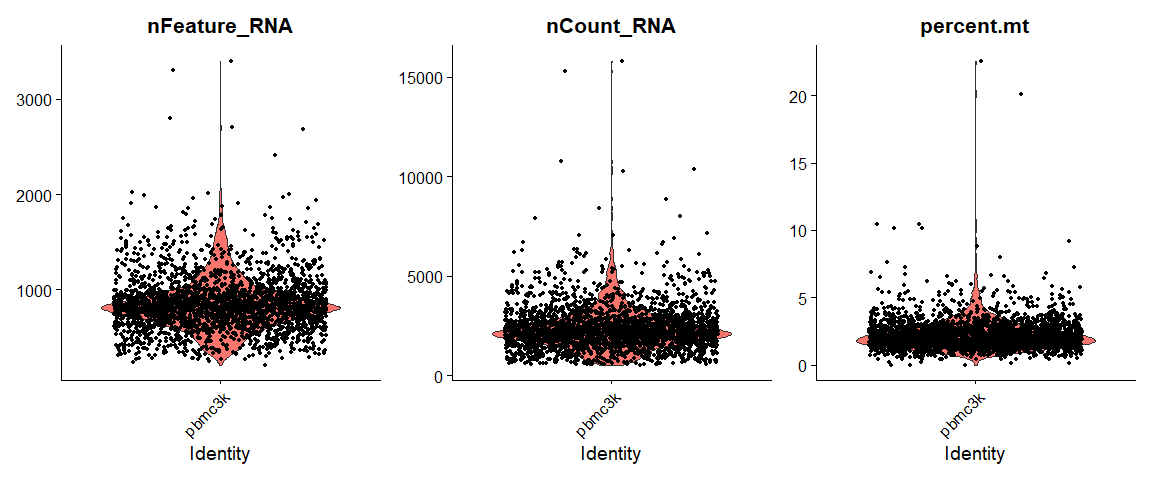
2.1 细胞质控
三种基本的QC metrics
- The number of unique genes detected in each cell.
- Low-quality cells or empty droplets will often have very few genes
- Cell doublets or multiplets may exhibit an aberrantly high gene count
- Similarly, the total number of molecules detected within a cell (correlates strongly with unique genes)
- The percentage of reads that map to the mitochondrial genome
- Low-quality / dying cells often exhibit extensive mitochondrial contamination
- We calculate mitochondrial QC metrics with the
PercentageFeatureSetfunction, which calculates the percentage of counts originating from a set of features- We use the set of all genes starting with
MT-as a set of mitochondrial genes
注意,人的线粒体基因是“MT-”开头,而小鼠的线粒体基因是“mt-”开头
# The [[ operator can add columns to object metadata. This is a great place to stash QC stats |
##                orig.ident nCount_RNA nFeature_RNA seurat_annotations percent.mt
## AAACATACAACCAC     pbmc3k       2419          779       Memory CD4 T  3.0177759
## AAACATTGAGCTAC     pbmc3k       4903         1352                  B  3.7935958
## AAACATTGATCAGC     pbmc3k       3147         1129       Memory CD4 T  0.8897363
## AAACCGTGCTTCCG     pbmc3k       2639          960         CD14+ Mono  1.7430845
## AAACCGTGTATGCG pbmc3k 980 521 NK 1.2244898由于我们用的是作者给了metadata的数据,里面已经出现了细胞类型的注释,见seurat_annotation这一项;
QC metric的可视化:
# Visualize QC metrics as a violin plot |
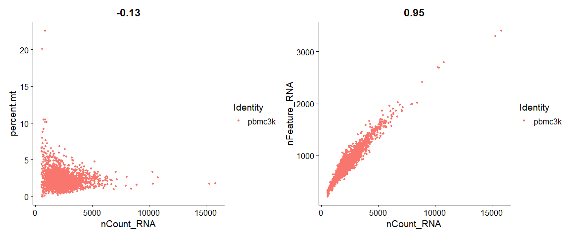
# FeatureScatter is typically used to visualize feature-feature relationships, but can be used |
最终选择的质控标准为:
- We filter cells that have unique feature counts over 2,500 or less than 200
- We filter cells that have >5% mitochondrial counts
pbmc <- subset(pbmc, subset = nFeature_RNA > 200 & nFeature_RNA < 2500 & percent.mt < 5) |
2.2 标准化
After removing unwanted cells from the dataset, the next step is to normalize the data. By default, we employ a global-scaling normalization method “LogNormalize” that normalizes the feature expression measurements for each cell by the total expression, multiplies this by a scale factor (10,000 by default), and log-transforms the result. Normalized values are stored in pbmc[[“RNA”]]@data.
pbmc <- NormalizeData(pbmc, normalization.method = "LogNormalize", scale.factor = 10000) |
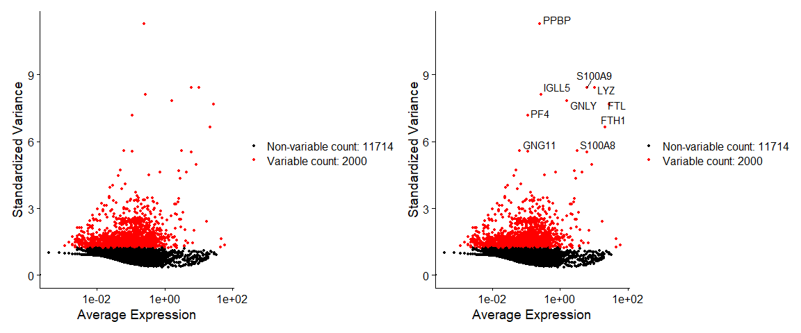
2.3 特征选择
哪些基因能反应不同细胞之间的异质性?是那些表达差异大的基因;
注意FindVariableFeatures是S3 generic,泛型函数。 如何查看一个泛型函数的源代码呢,我们先用methods函数匹配该范型函数的名字:
methods(FindVariableFeatures) |
## [1] FindVariableFeatures.Assay*   FindVariableFeatures.default*
## [3] FindVariableFeatures.Seurat*
## see '?methods' for accessing help and source code
星号表明我们不能直接通过运行函数名字来查看其源代码,但是我们可以通过运行 getAnywhere函数来获取这个函数,
getAnywhere(FindVariableFeatures.Seurat) |
## A single object matching 'FindVariableFeatures.Seurat' was found
## It was found in the following places
##   registered S3 method for FindVariableFeatures from namespace Seurat
##   namespace:Seurat
## with value
##
## function (object, assay = NULL, selection.method = "vst", loess.span = 0.3,
##     clip.max = "auto", mean.function = FastExpMean, dispersion.function = FastLogVMR,
##     num.bin = 20, binning.method = "equal_width", nfeatures = 2000,
##     mean.cutoff = c(0.1, 8), dispersion.cutoff = c(1, Inf), verbose = TRUE,
##     ...)
## {
##     assay <- assay %||% DefaultAssay(object = object)
##     assay.data <- GetAssay(object = object, assay = assay)
##     assay.data <- FindVariableFeatures(object = assay.data, selection.method = selection.method,
##         loess.span = loess.span, clip.max = clip.max, mean.function = mean.function,
##         dispersion.function = dispersion.function, num.bin = num.bin,
##         binning.method = binning.method, nfeatures = nfeatures,
##         mean.cutoff = mean.cutoff, dispersion.cutoff = dispersion.cutoff,
##         verbose = verbose, ...)
##     object[[assay]] <- assay.data
##     object <- LogSeuratCommand(object = object)
##     return(object)
## }
## <bytecode: 0x0000000022fa2410>
## <environment: namespace:Seurat>我们可以发现,默认的FindVariableFeatures.Seuratmethod调用了FindVariableFeatures.Assay:
getAnywhere(FindVariableFeatures.Assay) |
## A single object matching 'FindVariableFeatures.Assay' was found
## It was found in the following places
##   registered S3 method for FindVariableFeatures from namespace Seurat
##   namespace:Seurat
## with value
##
## function (object, selection.method = "vst", loess.span = 0.3,
##     clip.max = "auto", mean.function = FastExpMean, dispersion.function = FastLogVMR,
##     num.bin = 20, binning.method = "equal_width", nfeatures = 2000,
##     mean.cutoff = c(0.1, 8), dispersion.cutoff = c(1, Inf), verbose = TRUE,
##     ...)
## {
##     if (length(x = mean.cutoff) != 2 || length(x = dispersion.cutoff) !=
##         2) {
##         stop("Both 'mean.cutoff' and 'dispersion.cutoff' must be two numbers")
##     }
##     if (selection.method == "vst") {
##         data <- GetAssayData(object = object, slot = "counts")
##         if (IsMatrixEmpty(x = data)) {
##             warning("selection.method set to 'vst' but count slot is empty; will use data slot instead")
##             data <- GetAssayData(object = object, slot = "data")
##         }
##     }
##     else {
##         data <- GetAssayData(object = object, slot = "data")
##     }
##     hvf.info <- FindVariableFeatures(object = data, selection.method = selection.method,
##         loess.span = loess.span, clip.max = clip.max, mean.function = mean.function,
##         dispersion.function = dispersion.function, num.bin = num.bin,
##         binning.method = binning.method, verbose = verbose, ...)
##     object[[names(x = hvf.info)]] <- hvf.info
##     hvf.info <- hvf.info[which(x = hvf.info[, 1, drop = TRUE] !=
##         0), ]
##     if (selection.method == "vst") {
##         hvf.info <- hvf.info[order(hvf.info$vst.variance.standardized,
##             decreasing = TRUE), , drop = FALSE]
##     }
##     else {
##         hvf.info <- hvf.info[order(hvf.info$mvp.dispersion, decreasing = TRUE),
##             , drop = FALSE]
##     }
##     selection.method <- switch(EXPR = selection.method, mvp = "mean.var.plot",
##         disp = "dispersion", selection.method)
##     top.features <- switch(EXPR = selection.method, mean.var.plot = {
##         means.use <- (hvf.info[, 1] > mean.cutoff[1]) & (hvf.info[,
##             1] < mean.cutoff[2])
##         dispersions.use <- (hvf.info[, 3] > dispersion.cutoff[1]) &
##             (hvf.info[, 3] < dispersion.cutoff[2])
##         rownames(x = hvf.info)[which(x = means.use & dispersions.use)]
##     }, dispersion = head(x = rownames(x = hvf.info), n = nfeatures),
##         vst = head(x = rownames(x = hvf.info), n = nfeatures),
##         stop("Unkown selection method: ", selection.method))
##     VariableFeatures(object = object) <- top.features
##     vf.name <- ifelse(test = selection.method == "vst", yes = "vst",
##         no = "mvp")
##     vf.name <- paste0(vf.name, ".variable")
##     object[[vf.name]] <- rownames(x = object[[]]) %in% top.features
##     return(object)
## }
## <bytecode: 0x000000002dc5d050>
## <environment: namespace:Seurat>
千层饼的最后一层;
getAnywhere(FindVariableFeatures.default) |
## A single object matching 'FindVariableFeatures.default' was found
## It was found in the following places
##   registered S3 method for FindVariableFeatures from namespace Seurat
##   namespace:Seurat
## with value
##
## function (object, selection.method = "vst", loess.span = 0.3,
##     clip.max = "auto", mean.function = FastExpMean, dispersion.function = FastLogVMR,
##     num.bin = 20, binning.method = "equal_width", verbose = TRUE,
##     ...)
## {
##     CheckDots(...)
##     if (!inherits(x = object, "Matrix")) {
##         object <- as(object = as.matrix(x = object), Class = "Matrix")
##     }
##     if (!inherits(x = object, what = "dgCMatrix")) {
##         object <- as(object = object, Class = "dgCMatrix")
##     }
##     if (selection.method == "vst") {
##         if (clip.max == "auto") {
##             clip.max <- sqrt(x = ncol(x = object))
##         }
##         hvf.info <- data.frame(mean = rowMeans(x = object))
##         hvf.info$variance <- SparseRowVar2(mat = object, mu = hvf.info$mean,
##             display_progress = verbose)
##         hvf.info$variance.expected <- 0
##         hvf.info$variance.standardized <- 0
##         not.const <- hvf.info$variance > 0
##         fit <- loess(formula = log10(x = variance) ~ log10(x = mean),
##             data = hvf.info[not.const, ], span = loess.span)
##         hvf.info$variance.expected[not.const] <- 10^fit$fitted
##         hvf.info$variance.standardized <- SparseRowVarStd(mat = object,
##             mu = hvf.info$mean, sd = sqrt(hvf.info$variance.expected),
##             vmax = clip.max, display_progress = verbose)
##         colnames(x = hvf.info) <- paste0("vst.", colnames(x = hvf.info))
##     }
##     else {
##         if (!inherits(x = mean.function, what = "function")) {
##             stop("'mean.function' must be a function")
##         }
##         if (!inherits(x = dispersion.function, what = "function")) {
##             stop("'dispersion.function' must be a function")
##         }
##         feature.mean <- mean.function(object, verbose)
##         feature.dispersion <- dispersion.function(object, verbose)
##         names(x = feature.mean) <- names(x = feature.dispersion) <- rownames(x = object)
##         feature.dispersion[is.na(x = feature.dispersion)] <- 0
##         feature.mean[is.na(x = feature.mean)] <- 0
##         data.x.breaks <- switch(EXPR = binning.method, equal_width = num.bin,
##             equal_frequency = c(-1, quantile(x = feature.mean[feature.mean >
##                 0], probs = seq.int(from = 0, to = 1, length.out = num.bin))),
##             stop("Unknown binning method: ", binning.method))
##         data.x.bin <- cut(x = feature.mean, breaks = data.x.breaks)
##         names(x = data.x.bin) <- names(x = feature.mean)
##         mean.y <- tapply(X = feature.dispersion, INDEX = data.x.bin,
##             FUN = mean)
##         sd.y <- tapply(X = feature.dispersion, INDEX = data.x.bin,
##             FUN = sd)
##         feature.dispersion.scaled <- (feature.dispersion - mean.y[as.numeric(x = data.x.bin)])/sd.y[as.numeric(x = data.x.bin)]
##         names(x = feature.dispersion.scaled) <- names(x = feature.mean)
##         hvf.info <- data.frame(feature.mean, feature.dispersion,
##             feature.dispersion.scaled)
##         rownames(x = hvf.info) <- rownames(x = object)
##         colnames(x = hvf.info) <- paste0("mvp.", c("mean", "dispersion",
##             "dispersion.scaled"))
##     }
##     return(hvf.info)
## }
## <bytecode: 0x0000000023f13fd0>
## <environment: namespace:Seurat>
忽略这些技术细节,进行特征选择;
pbmc <- FindVariableFeatures(pbmc, selection.method = "vst", nfeatures = 2000) |
2.4 Scaling the data
这步的目的是为了后续的PCA:
Next, we apply a linear transformation (‘scaling’) that is a standard pre-processing step prior to dimensional reduction techniques like PCA. The ScaleData function: + Shifts the expression of each gene, so that the mean expression across cells is 0 + Scales the expression of each gene, so that the variance across cells is 1 + This step gives equal weight in downstream analyses, so that highly-expressed genes do not dominate + The results of this are stored in pbmc[[“RNA”]]@scale.data
回归掉percent.mt对于PCA的影响。这步是一步限速步骤;
all.genes <- rownames(pbmc) |
有一个问题后面的marker基因一定是HVG吗?
2.5 线性降维(PCA)
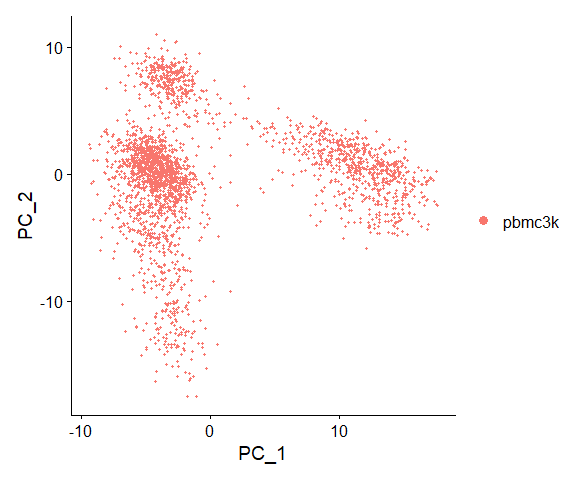
Next we perform PCA on the scaled data. By default, only the previously determined variable features are used as input, but can be defined using features argument if you wish to choose a different subset.
pbmc <- RunPCA(pbmc, features = VariableFeatures(object = pbmc)) |
## PC_ 1
## Positive:  CST3, TYROBP, LST1, AIF1, FTL
## Negative:  MALAT1, LTB, IL32, IL7R, CD2
## PC_ 2
## Positive:  CD79A, MS4A1, TCL1A, HLA-DQA1, HLA-DQB1
## Negative:  NKG7, PRF1, CST7, GZMA, GZMB
## PC_ 3
## Positive:  HLA-DQA1, CD79A, CD79B, HLA-DQB1, HLA-DPA1
## Negative:  PPBP, PF4, SDPR, SPARC, GNG11
## PC_ 4
## Positive:  HLA-DQA1, CD79B, CD79A, MS4A1, HLA-DQB1
## Negative:  VIM, IL7R, S100A6, S100A8, IL32
## PC_ 5
## Positive:  GZMB, FGFBP2, S100A8, NKG7, GNLY
## Negative: LTB, IL7R, CKB, MS4A7, RP11-290F20.3VizDimLoadings(pbmc, dims = 1:2, reduction = "pca") |

DimPlot(pbmc, reduction = "pca") |
In particular DimHeatmap allows for easy exploration of the primary sources of heterogeneity in a dataset, and can be useful when trying to decide which PCs to include for further downstream analyses. Both cells and features are ordered according to their PCA scores. Setting cells to a number plots the ‘extreme’ cells on both ends of the spectrum, which dramatically speeds plotting for large datasets. Though clearly a supervised analysis, we find this to be a valuable tool for exploring correlated feature sets.
### Plot an equal number of genes with both + and - scores. |
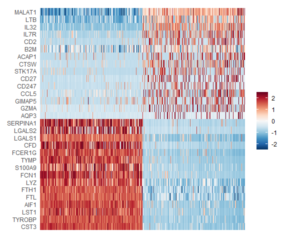
DimHeatmap(pbmc, dims = 1:15, cells = 500, balanced = TRUE) |

2.6 Determine the ‘dimensionality’ of the dataset
To overcome the extensive technical noise in any single feature for scRNA-seq data, Seurat clusters cells based on their PCA scores, with each PC essentially representing a ‘metafeature’ that combines information across a correlated feature set. The top principal components therefore represent a robust compression of the dataset. However, how many componenets should we choose to include? 10? 20? 100?
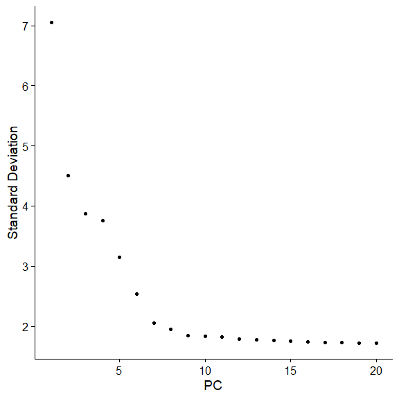
两种统计方法,JackStraw和ElbowPlot,前者比较耗时,不再展示了,用后者
ElbowPlot(pbmc) |
作者给出了更进一步的解释
Identifying the true dimensionality of a dataset – can be challenging/uncertain for the user. We therefore suggest these three approaches to consider. The first is more supervised, exploring PCs to determine relevant sources of heterogeneity, and could be used in conjunction with GSEA for example. The second implements a statistical test based on a random null model, but is time-consuming for large datasets, and may not return a clear PC cutoff. The third is a heuristic that is commonly used, and can be calculated instantly. In this example, all three approaches yielded similar results, but we might have been justified in choosing anything between PC 7-12 as a cutoff.
We chose 10 here, but encourage users to consider the following:
- Dendritic cell and NK aficionados may recognize that genes strongly associated with PCs 12 and 13 define rare immune subsets (i.e. MZB1 is a marker for plasmacytoid DCs). However, these groups are so rare, they are difficult to distinguish from background noise for a dataset of this size without prior knowledge.
- We encourage users to repeat downstream analyses with a different number of PCs (10, 15, or even 50!). As you will observe, the results often do not differ dramatically.
- We advise users to err on the higher side when choosing this parameter. For example, performing downstream analyses with only 5 PCs does signifcanltly and adversely affect results.
3. 后续分析
3.1 聚类
FindNeighbors构建构建SNN-graph, 而FindClusters用来实现Louvain algorithm,进行图聚类;
methods(FindNeighbors) |
## [1] FindNeighbors.Assay*   FindNeighbors.default* FindNeighbors.dist*
## [4] FindNeighbors.Seurat*
## see '?methods' for accessing help and source codegetAnywhere(FindNeighbors.Seurat) |
## A single object matching 'FindNeighbors.Seurat' was found
## It was found in the following places
##   registered S3 method for FindNeighbors from namespace Seurat
##   namespace:Seurat
## with value
##
## function (object, reduction = "pca", dims = 1:10, assay = NULL,
##     features = NULL, k.param = 20, compute.SNN = TRUE, prune.SNN = 1/15,
##     nn.method = "rann", annoy.metric = "euclidean", nn.eps = 0,
##     verbose = TRUE, force.recalc = FALSE, do.plot = FALSE, graph.name = NULL,
##     ...)
## {
##     CheckDots(...)
##     if (!is.null(x = dims)) {
##         assay <- DefaultAssay(object = object[[reduction]])
##         data.use <- Embeddings(object = object[[reduction]])
##         if (max(dims) > ncol(x = data.use)) {
##             stop("More dimensions specified in dims than have been computed")
##         }
##         data.use <- data.use[, dims]
##         neighbor.graphs <- FindNeighbors(object = data.use, k.param = k.param,
##             compute.SNN = compute.SNN, prune.SNN = prune.SNN,
##             nn.method = nn.method, annoy.metric = annoy.metric,
##             nn.eps = nn.eps, verbose = verbose, force.recalc = force.recalc,
##             ...)
##     }
##     else {
##         assay <- assay %||% DefaultAssay(object = object)
##         data.use <- GetAssay(object = object, assay = assay)
##         neighbor.graphs <- FindNeighbors(object = data.use, features = features,
##             k.param = k.param, compute.SNN = compute.SNN, prune.SNN = prune.SNN,
##             nn.method = nn.method, annoy.metric = annoy.metric,
##             nn.eps = nn.eps, verbose = verbose, force.recalc = force.recalc,
##             ...)
##     }
##     graph.name <- graph.name %||% paste0(assay, "_", names(x = neighbor.graphs))
##     for (ii in 1:length(x = graph.name)) {
##         DefaultAssay(object = neighbor.graphs[[ii]]) <- assay
##         object[[graph.name[[ii]]]] <- neighbor.graphs[[ii]]
##     }
##     if (do.plot) {
##         if (!"tsne" %in% names(x = object@reductions)) {
##             warning("Please compute a tSNE for SNN visualization. See RunTSNE().")
##         }
##         else {
##             if (nrow(x = Embeddings(object = object[["tsne"]])) !=
##                 ncol(x = object)) {
##                 warning("Please compute a tSNE for SNN visualization. See RunTSNE().")
##             }
##             else {
##                 net <- graph.adjacency(adjmatrix = as.matrix(x = neighbor.graphs[[2]]),
##                   mode = "undirected", weighted = TRUE, diag = FALSE)
##                 plot.igraph(x = net, layout = as.matrix(x = Embeddings(object = object[["tsne"]])),
##                   edge.width = E(graph = net)$weight, vertex.label = NA,
##                   vertex.size = 0)
##             }
##         }
##     }
##     object <- LogSeuratCommand(object = object)
##     return(object)
## }
## <bytecode: 0x000000001e49f8e0>
## <environment: namespace:Seurat>
pbmc <- FindNeighbors(pbmc, dims = 1:10) |
## Modularity Optimizer version 1.3.0 by Ludo Waltman and Nees Jan van Eck
##
## Number of nodes: 2638
## Number of edges: 95930
##
## Running Louvain algorithm...
## Maximum modularity in 10 random starts: 0.8737
## Number of communities: 9
## Elapsed time: 0 seconds
3.2 Run UMAP/tsne
run tsne
pbmc <- RunTSNE(pbmc,dims = 1:10) |
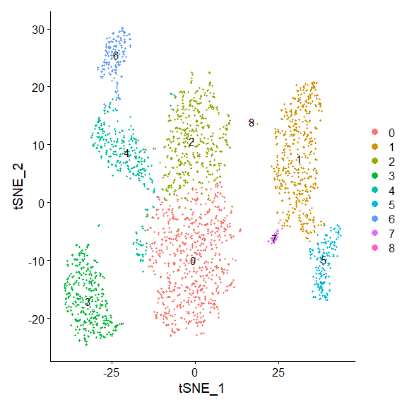
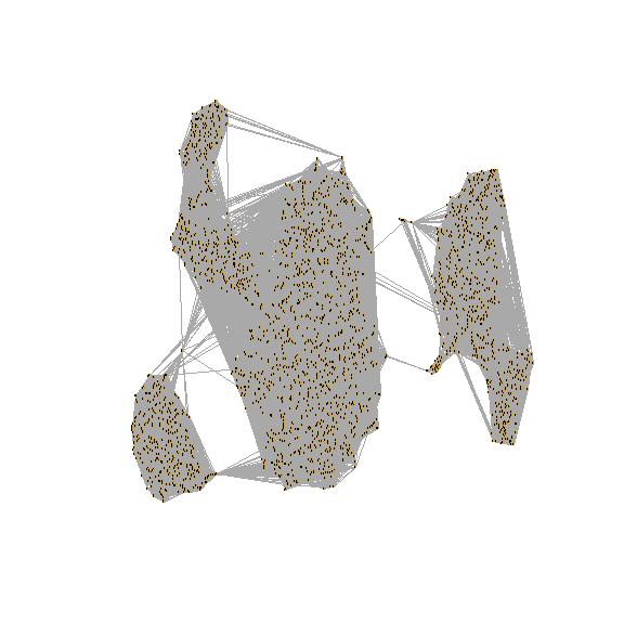
draw snn graph on tsne-embeding
test <- pbmc[["RNA_snn"]] |
run umap
# If you haven't installed UMAP, you can do so via reticulate::py_install(packages = |

test <- pbmc[["RNA_snn"]] |
3.3 Finding differentially expressed features (cluster biomarkers)
之前分群结果做差异表达;
Seurat can help you find markers that define clusters via differential expression. By default, it identifes positive and negative markers of a single cluster (specified in ident.1), compared to all other cells. FindAllMarkers automates this process for all clusters, but you can also test groups of clusters vs. each other, or against all cells.
The min.pct argument requires a feature to be detected at a minimum percentage in either of the two groups of cells, and the thresh.test argument requires a feature to be differentially expressed (on average) by some amount between the two groups. You can set both of these to 0, but with a dramatic increase in time - since this will test a large number of features that are unlikely to be highly discriminatory. As another option to speed up these computations, max.cells.per.ident can be set. This will downsample each identity class to have no more cells than whatever this is set to. While there is generally going to be a loss in power, the speed increases can be significiant and the most highly differentially expressed features will likely still rise to the top.
# find markers for every cluster compared to all remaining cells, report only the positive ones |
## # A tibble: 18 x 7
## # Groups: cluster [9]
## p_val avg_logFC pct.1 pct.2 p_val_adj cluster gene
## <dbl> <dbl> <dbl> <dbl> <dbl> <fct> <chr>
## 1 1.88e-117 0.748 0.913 0.588 2.57e-113 0 LDHB
## 2 5.01e- 85 0.931 0.437 0.108 6.88e- 81 0 CCR7
## 3 0. 3.86 0.996 0.215 0. 1 S100A9
## 4 0. 3.80 0.975 0.121 0. 1 S100A8
## 5 2.61e- 81 0.886 0.981 0.65 3.58e- 77 2 LTB
## 6 1.22e- 59 0.886 0.669 0.25 1.68e- 55 2 CD2
## 7 0. 2.99 0.939 0.042 0. 3 CD79A
## 8 1.06e-269 2.49 0.623 0.022 1.45e-265 3 TCL1A
## 9 5.98e-221 2.23 0.987 0.226 8.20e-217 4 CCL5
## 10 1.42e-173 2.08 0.572 0.051 1.94e-169 4 GZMK
## 11 3.51e-184 2.30 0.975 0.134 4.82e-180 5 FCGR3A
## 12 2.03e-125 2.14 1 0.315 2.78e-121 5 LST1
## 13 3.17e-267 3.35 0.961 0.068 4.35e-263 6 GZMB
## 14 1.04e-189 3.66 0.961 0.132 1.43e-185 6 GNLY
## 15 1.48e-220 2.68 0.812 0.011 2.03e-216 7 FCER1A
## 16 1.67e- 21 1.99 1 0.513 2.28e- 17 7 HLA-DPB1
## 17 7.73e-200 5.02 1 0.01 1.06e-195 8 PF4
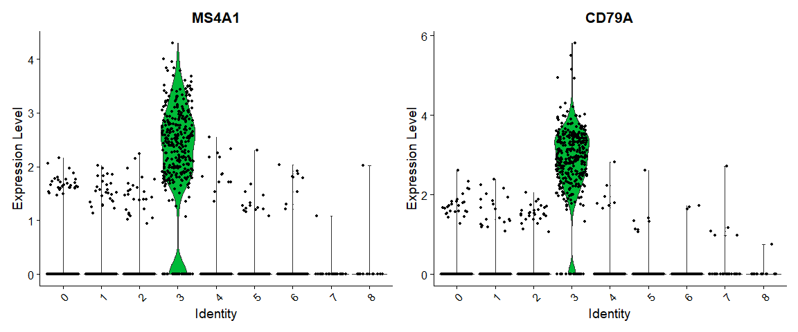
## 18 3.68e-110 5.94 1 0.024 5.05e-106 8 PPBP可视化:
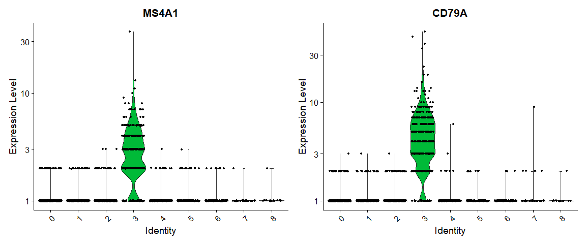
VlnPlot(pbmc, features = c("MS4A1", "CD79A")) |
# you can plot raw counts as well |
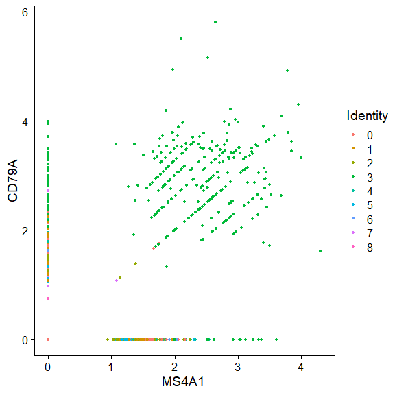
使用FeatureScatter获得和流式图一样的效果;
FeatureScatter(object = pbmc, |
用FeaturePlot在Embeding上展示表达量;
FeaturePlot(pbmc, features = c("MS4A1", "GNLY", "CD3E", "CD14", "FCER1A", "FCGR3A", "LYZ", "PPBP", |

气泡图DotPlot
DotPlot(object = pbmc, |

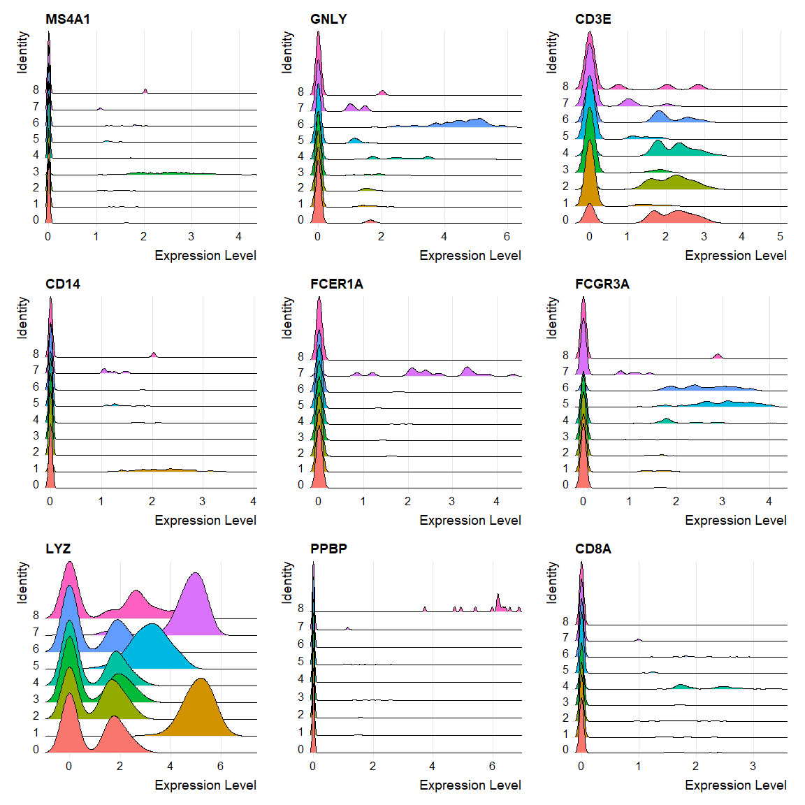
RidgePlot
RidgePlot(object = pbmc, |
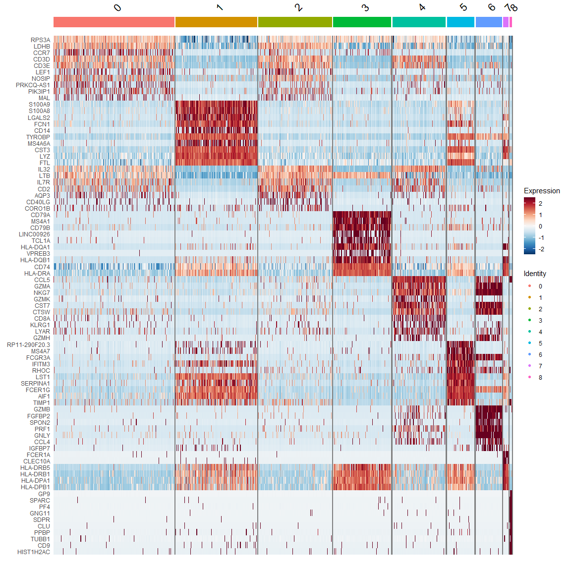
热图DoHeatmap
top10 <- pbmc.markers %>% |
3.4 Assigning cell type identity to clusters
new.cluster.ids <- c("Naive CD4 T","CD14+ Mono", "Memory CD4 T", "B", "CD8 T", "FCGR3A+ Mono", "NK", "DC", "Platelet") |

4. Seurat object 详解
这一部分来自wiki
4.1 The Seurat object
一个Seurat对象有如下的slots:
| Slot | Function |
|---|---|
assays |
A list of assays within this object |
meta.data |
Cell-level meta data |
active.assay |
Name of active, or default, assay |
active.ident |
Identity classes for the current object |
graphs |
A list of nearest neighbor graphs |
reductions |
A list of DimReduc objects |
project.name |
User-defined project name (optional) |
tools |
Empty list. Tool developers can store any internal data from their methods here |
misc |
Empty slot. User can store additional information here |
version |
Seurat version used when creating the object |
这个对象把单细胞数据的所有的基本信息都包含进去了,可以用基本的一些函数去获取这些信息。例如,我们想要知道这个数据对应多少细胞,多少基因,可以用dim;ncol;nrow;细胞或者feature的名字,可以用rownames;colnames; 我们也可以通过names知道里面存储的如原始表达矩阵,或者降维后对象的名字。
names(x = pbmc) |
## [1] "RNA" "RNA_nn" "RNA_snn" "pca" "tsne" "umap"rna <- pbmc[['RNA']] |
对于Seurat对象,有一系列的函数可以对其进行操作。这些函数可以称为其所属的methods。多说一句,Seurat采取的是S3对象的面向对象的数据结构。
可以使用如下命令访问与Seurat对象相关的操作。
utils::methods(class = 'Seurat') |
##  [1] $                       $<-                     [
##  [4] [[                      [[<-                    AddMetaData
##  [7] as.CellDataSet          as.loom                 as.SingleCellExperiment
## [10] Command                 DefaultAssay            DefaultAssay<-
## [13] dim                     dimnames                droplevels
## [16] Embeddings              FindClusters            FindMarkers
## [19] FindNeighbors           FindVariableFeatures    GetAssay
## [22] GetAssayData            HVFInfo                 Idents
## [25] Idents<-                Key                     levels
## [28] levels<-                Loadings                merge
## [31] Misc                    Misc<-                  names
## [34] NormalizeData           OldWhichCells           Project
## [37] Project<-               RenameCells             RenameIdents
## [40] ReorderIdent            RunALRA                 RunCCA
## [43] RunICA                  RunLSI                  RunPCA
## [46] RunTSNE                 RunUMAP                 ScaleData
## [49] ScoreJackStraw          SetAssayData            SetIdent
## [52] show                    StashIdent              Stdev
## [55] subset                  SubsetData              Tool
## [58] Tool<-                  VariableFeatures        VariableFeatures<-
## [61] WhichCells
## see '?methods' for accessing help and source code
4.2 Assay
The
Assayclass stores single cell data.
For typical scRNA-seq experiments, a Seurat object will have a single Assay (“RNA”). This assay will also store multiple ‘transformations’ of the data, including raw counts (@counts slot), normalized data (@data slot), and scaled data for dimensional reduction (@scale.data slot).
For more complex experiments, an object could contain multiple assays. These could include multi-modal data types (CITE-seq antibody-derived tags, ADTs), or imputed/batch-corrected measurements. Each of those assays has the option to store the same data transformations as well.
一个Assay 所含有的Slots
| Slot | Function |
|---|---|
counts |
Stores unnormalized data such as raw counts or TPMs |
data |
Normalized data matrix |
scale.data |
Scaled data matrix |
key |
A character string to facilitate looking up features from a specific Assay |
var.features |
A vector of features identified as variable |
meta.features |
Feature-level meta data |
Assay对象也可以使用以下方法
Summary information about Assay objects can be had quickly and easily using standard R functions. Object shape/dimensions can be found using the dim, ncol, and nrow functions; cell and feature names can be found using the colnames and rownames functions, respectively, or the dimnames function.
更多的方法见
utils::methods(class = 'Assay') |
##  [1] [                    [[                   [[<-
##  [4] AddMetaData          DefaultAssay         DefaultAssay<-
##  [7] dim                  dimnames             FindNeighbors
## [10] FindVariableFeatures GetAssayData         HVFInfo
## [13] Key                  Key<-                merge
## [16] Misc                 Misc<-               NormalizeData
## [19] OldWhichCells        RenameCells          RunICA
## [22] RunLSI               RunPCA               ScaleData
## [25] SetAssayData         show                 subset
## [28] SubsetData           VariableFeatures     VariableFeatures<-
## [31] WhichCells
## see '?methods' for accessing help and source code
Data Access
# GetAssayData allows pulling from a specific slot rather than just data |
##               AAACATACAACCAC AAACATTGAGCTAC AAACATTGATCAGC
## AL627309.1       -0.06433822    -0.06968772    -0.04966479
## AP006222.2       -0.02663018    -0.02065038    -0.04303249
## RP11-206L10.2 -0.03015459 -0.02024084 -0.05734758head(x = HVFInfo(object = rna,selection.method = "vst")) |
##                      mean    variance variance.standardized
## AL627309.1    0.003411676 0.003401325             0.9330441
## AP006222.2    0.001137225 0.001136363             0.9924937
## RP11-206L10.2 0.001895375 0.001892500             0.9627290
## RP11-206L10.9 0.001137225 0.001136363             0.9924937
## LINC00115     0.006823351 0.006779363             0.9062135
## NOC2L         0.107278241 0.159514698             0.7849309
The key
# Key both accesses and sets the key slot for an Assay object |
The DimReduc object represents a dimensional reduction taken upon the Seurat object.
4.3 The DimReduc object
The DimReduc object represents a dimensional reduction taken upon the Seurat object.
| Slot | Function |
|---|---|
cell.embeddings |
A matrix with cell embeddings |
feature.loadings |
A matrix with feature loadings |
feature.loadings.projected |
A matrix with projected feature loadings |
assay.used |
Assay used to calculate this dimensional reduction |
stdev |
Standard deviation for the dimensional reduction |
key |
A character string to facilitate looking up features from a specific DimReduc |
jackstraw |
Results from the JackStraw function |
misc |
… |
和之前的很类似
pca <- pbmc[["pca"]] |
Access data
# The key can be used to pull cell embeddings for specific dimensions from the Seurat level |
在其上可以执行的method有
utils::methods(class = "DimReduc") |
##  [1] [              [[             Cells          DefaultAssay   DefaultAssay<-
##  [6] dim            dimnames       Embeddings     IsGlobal       JS
## [11] JS<-           Key            Key<-          length         Loadings
## [16] Loadings<-     names          print          RenameCells    RunTSNE
## [21] ScoreJackStraw show           Stdev          subset
## see '?methods' for accessing help and source code
4.4 R面向对象编程的更多细节;
关于面向对象,以及S3对象的教程,更多可见: